Who should read it
Anyone interested in programming or to learn about predator-prey dynamics.
Fun with Predator-Prey Models: A Programming Exercise
There are definitely better versions of predator-prey models available online, especially some AI-based versions that are quite interesting. However, I think that the most simple version, which we study here, is a good starting point to delve into the subject. For non-expert programmers, it already poses some difficult yet solvable questions. For a mathematical explanation of the subject have a look at the Lotka-Volterra equations.
How it works
In this simulation, wolves and sheep roam randomly around a landscape. Wolves are predators, and they hunt down sheep to feed on. However, each step they take requires energy, which can only be replenished by consuming a sheep. If a wolf runs out of energy, it dies. In order to maintain a stable population, each wolf and sheep has a fixed probability of reproducing at each time step. Unlike wolves, sheep do not gain or lose energy from eating or moving, as we assume that grass is always available for them to eat.
Initializing the model
# set the size of the world (100x100 grid)
world_size = 100

# set the initial number of sheep and wolves
initial_n_sheep = 100
initial_n_wolves = 50

# set the reproduction rates of sheep and wolves, respectively
sheep_reproduction = 0.04
wolves_reproduction = 0.05

# define how much energy wolves gain when they find prey
wolves_gain  = 20

# define how much energy wolves loose for each step they make
wolves_loose = 2

# define energy of new born wolves
energy_new_borns = 20

# energy cannot exceed 40
max_energy = 40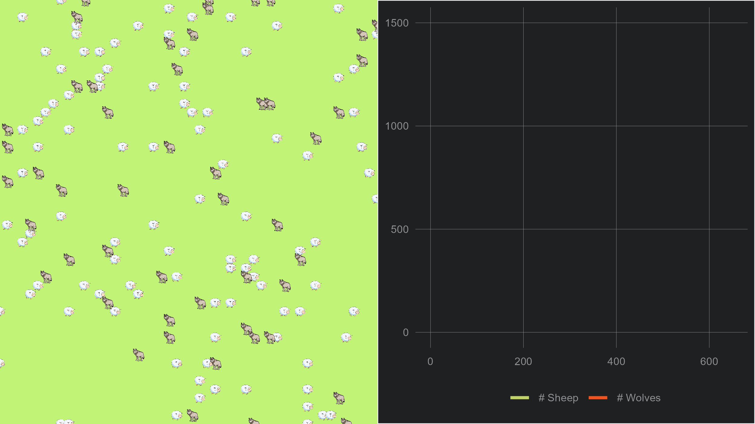
While the model is simple, it requires several parameters to function properly. We then let the model run with these settings. The left panel of the animation shows the movement of wolves and sheep in our square world. On the right side of the screen, we document the total number of sheep and wolves over time. We are interested in the overall predator-prey dynamics. Pause here for a moment to describe the potential dynamics of this system.
Results
At first, there may be more sheep than wolves, so the wolves have plenty of food and their population grows. As the wolf population grows, they catch more and more sheep, which causes the sheep population to decline. With fewer sheep, there is less food for the wolves, and their population starts to decline as well.
As the wolf population declines, there are fewer predators to hunt the sheep, so the sheep population starts to grow again. With more sheep, the wolves have more food available, so their population starts to grow again as well. And so the cycle continues. In our simple model, the population dynamics are ultimately unstable. In this example, after the second cycle only sheep survive. However, if we would run the same model again, with a different seed, wolves may be the surviving species.
In general, it is difficult to predict which of the two species will survive in the predator-prey dynamics without examining the specific parameters and initial conditions of the simulation. The population dynamics of the wolves and sheep will depend on factors such as their reproductive rates, and energy costs and gains. Additionally, chance events such as random encounters and deaths can also play a role.
Exercise
- Use the model explanation from above and try to code it on your own before looking at the code in the appendix below.
- Improve the code below either by speeding up the calculations or by reducing the number of lines (e.g. is it possible to use R’s power of vectorization instead of the loop?).
Appendix: Code
Below you will find the code used to create the animation above. It
is not intended to be the most efficient or practical implementation, as
that is left up to you (see exercise 2). However, I utilized the
data.table package as it allows for more efficient data transformation.
If you are unfamiliar with the package, it is worth taking the time to
learn about it.
library( data.table )
library( ggimage )
library( ggplot2)
set.seed( 20230510 )

# set up project paths
MAIN_PATH <- dirname( rstudioapi::getActiveDocumentContext()$path )
DATA      <- file.path( MAIN_PATH, "data" )

if( !dir.exists( DATA ) ) dir.create( DATA )

# initialize model
  world_size <- 50
  initial_n_sheeps <- 100
  initial_n_wolves <- 50
  sheeps_reproduction <- 0.04
  wolves_reproduction <- 0.05
  wolves_gain  <- 20 # wolves gain 0.2 of energy for each sheep they eat
  wolves_loose <- 2 # this basically means that wolves can make ten steps without
  # finding prey before they die.
  # set energy of new born wolves to 20
  energy_new_borns <- 20
  max_energy <- 40
  max_time <- 100

# create an empty raster (in long format)
  world <- data.table( row_idx = rep( 1:world_size, world_size ),
                       col_idx = rep( 1:world_size, each = world_size ),
                       agent   = 0 )
  world[ , row_col:=paste( row_idx, col_idx ) ]

# create a data.frame with the maximum number of agents
  agents <- data.table( type    = rep( 0, initial_n_sheeps + initial_n_wolves ),
                        energy  = numeric(),
                        row_idx = numeric(),
                        col_idx = numeric(),
                        row_col = character() )

  # initialize populations (position sheeps and wolves randomly in the world)
  idx <- sample( seq_len( nrow( world ) ), initial_n_sheeps + initial_n_wolves )

  agents[ 1:length( idx ), c( "row_idx", "col_idx", "row_col" ):= world[ idx, c( "row_idx", "col_idx", "row_col" ) ] ]
  agents[ 1:length( idx ), energy:=sample( seq( 2, 40, 1 ), size = length( idx ), replace = T) ]
  agents[ 1:length( idx ), type:=c( rep( 1, initial_n_sheeps ), rep( 2, initial_n_wolves ) ) ]

# create data.frame to store current states of the model
  df_states <- data.table( time = 1:max_time,
                           nSheeps = numeric(),
                           nWolves = numeric(),
                           averageWolfEnergy = numeric() )

  df_states[ 1, nSheeps:=initial_n_sheeps ]
  df_states[ 1, nWolves:=initial_n_wolves ]


  # populate grid
  x <- agents[ type == 1, row_col ]
  world[ row_col %chin% x, agent:=1 ]
  x <- agents[ type == 2, row_col ]
  world[ row_col %chin% x, agent:=2 ]

  # save grid
  saveRDS( world, file = paste0( DATA, "/world_grid_", 1, ".RDS" ) )

  world[ , agent:=0 ]

for( STEP in 2:max_time ){

  print( STEP )

  # reproduction sheeps (add new sheeps, no movement yet)
    new_agents <- c( sample( c( 0, 1 ),
                              size = nrow( agents[ type == 1 ] ),
                              replace = T,
                              prob = c( 1-sheeps_reproduction, sheeps_reproduction ) ),
                      sample( c( 0, 1 ),
                              size = nrow( agents[ type == 2 ] ),
                              replace = T,
                              prob = c( 1-wolves_reproduction, wolves_reproduction ) ) )

    new_agents <- agents[ as.logical( new_agents ), ]


    # force agents to new positions if no possible position is free agents can't be born
    new_agents[ , c( "row_idx", "col_idx" ) ] <- as.data.frame( t( apply( new_agents[ , c( "row_idx", "col_idx" ) ], 1, function( x ){

      temp <- paste( rep( x[ 1 ] + c( -1, 0, 1 ), 3 ), rep( x[ 2 ] + c( -1, 0, 1 ), each = 3 ) )

      out <- temp[ !temp %chin% agents$row_col ]

      if( length( out ) > 0 ){

        out <- as.numeric( unlist( strsplit( sample( out, 1 ), " " ) ) )

        out <- ifelse( out < 1, world_size, ifelse( out > world_size, 1, out ) )

      } else {

        out <- c( NA, NA )

      }

    } ) ) )

    # remove sheeps/wolves that did not find a free place
    new_agents <- na.omit( new_agents )

    new_agents[ , row_col:=paste( row_idx, col_idx ) ]
    # set energy of new born wolves to 20
    new_agents[ , energy:=energy_new_borns ]
    if( nrow( new_agents ) + nrow( agents ) < nrow( world ) ) agents <- rbindlist( list( agents, new_agents ) )

  # move all agents
    agents[ , row_idx:=row_idx+sample( c( -1, 0, 1 ), nrow( agents ), replace = T ) ]
    agents[ , col_idx:=col_idx+sample( c( -1, 0, 1 ), nrow( agents ), replace = T ) ]

  # adjust indices outside grid (world)
    agents[ row_idx < 1, row_idx:=world_size ]
    agents[ row_idx > world_size, row_idx:=1 ]
    agents[ col_idx < 1, col_idx:=world_size ]
    agents[ col_idx > world_size, col_idx:=1 ]
    agents[ , row_col:= paste( row_idx, col_idx ) ]
  # reduce energy of wolves
    agents[ type == 2, energy:=energy-wolves_loose ]

    # find wolves that found prey
    x <- agents[ type == 2, row_col ]
    wolves_eat <- x[ x %chin% agents[ type == 1, row_col ] ]
    # adjust energy
    agents[ type == 2 & row_col %chin% wolves_eat, energy:=energy+wolves_gain ]
    agents[ energy > max_energy, energy:=max_energy ]

    # remove sheeps that got eaten
    agents <- agents[ type == 2 | ( type == 1 & !row_col %chin% wolves_eat ) ]
    # remove wolves that died (energy = 0)
    agents <- agents[ type == 1  | ( energy > 0 & type == 2 ), ]

    df_states[ STEP, c( "nSheeps", "nWolves", "averageWolfEnergy" ):= data.frame( nrow( agents[ type == 1 ]), nrow( agents[ type == 2 ]), agents[ type == 2, mean( energy ) ] ) ]

  # populate grid
    x <- agents[ type == 1, row_col ]
    world[ row_col %chin% x, agent:=1 ]
    x <- agents[ type == 2, row_col ]
    world[ row_col %chin% x, agent:=2 ]

  # save grid
    saveRDS( world, file = paste0( DATA, "/world_grid_", STEP, ".RDS" ) )

    world[ , agent:=0 ]

}

# plot population
ggplot( tidyr::pivot_longer( df_states, -time ), aes( x = time, y = value, color = name ) ) + geom_line()

# plot populated world
df_plot <- readRDS( paste0( DATA, "/world_grid_", 50, ".RDS" ) )
df_plot[ , image:=ifelse( agent == 1, "lamb.png", ifelse( agent == 2, "wolf.png", NA ) ) ]
ggplot( df_plot, aes( x = col_idx, y = row_idx ) ) +
  geom_image(aes(image=image), size=.03) +
  # scale_fill_manual( values = my_cols ) +
  scale_y_continuous( expand = c( 0, 0 ) ) +
  scale_x_continuous( expand = c( 0, 0 ) ) +
  theme( axis.title = element_blank(),
         axis.text = element_blank(),
         legend.position = "none",
         panel.grid = element_blank(),
         axis.ticks = element_blank(),
         plot.margin=grid::unit(c(0,0,-1,-1), "mm"),
         panel.background = element_rect( fill = "#C1F376"))